Introduction
This final project is based around the Open Psychometrics “Which Character” Quiz. The quiz follows a standard internet format: Respondents assess themselves on series of opposed traits (e.g., are you more selfish or altruistic?), and at the end of the quiz, they are presented with their most similar fictional character (e.g., Batman or Buffy the Vampire Slayer). After the quiz has been completed, users are invited to rate the personalities of the characters themselves (e.g., is Batman more altruistic or selfish?). Open Psychometrics researchers have aggregated the ratings of 2,125 characters across 500 dimensions on a 100-point scale. The aggregate ratings are based on 3,386,031 user responses. Our work is inspired by the work of the Vermont Computational Story Lab, whose forthcoming work using the same data Dodds, 2025 deals with a long-debated question: Are there universal archetypes in fictional media?
Our goal is to explore patterns in the data and investigate associations that may suggest deeper cultural norms about how certain categories of people are depicted in fiction. Previous sociological work has focused on the importance of representation in shaping cultural perceptions Ramasubramanian et al., 2023, and such work has leveraged traditional content and media analysis. Studies on queer representation have discussed how gender- and sexuality-non-conforming characters are often positioned in narrow, repetitive roles Rodriguez, 2019, while decades of research on gender representation shows that the representation of women has improved to be less stereotyped—though issues of sexualization persist Mendes & Carter, 2008. Novel work has advocated for scholars to recognize age as also deeply culturally encoded Johfre, 2020. Meanwhile, nascent computation work both introduced word embeddings into the sociological discipline and assessed how class representations have shifted over time Kozlowski et al., 2019; still, lower classes are still degraded and stigmatized. Based on this work, we will investigate the straight_queer, young_old, masculine_feminine, and rich_poor demographic categories. By categorizing characters based on respondents’ ratings on these dimensions, we are assessing how perceptions of these categories are related to perceptions of other dimensions. Lastly, we will identify key potential archetypes with a mixture of principal component analysis (PCA), Gaussian mixture model (GMM), and hierarchical agglomerative clustering (HAC).
Data Description
The dataset characters-aggregated-scores.csv was downloaded from Open Psychometrics. Supplemental datasets called variable-key.csv and character-key.csv (to provide variable and character names) were developed based on the online documentation, which is available here as an .html file in the data folder. Note: If downloading an updated version of the dataset, the data formats, character names, and variables might have changed.
The characters-aggregated-scores.csv has 2125 rows, 501 columns which include an id column which is an object data type and BAP# ratings, and no missing values. The variable-key.csv data set provides information about what the BAP# columns correspond to in terms of adjective pairs for the ratings. The character-key.csv provides information on the id column relating each row to the character and movie/novel source for that character.
The BAP# ratings are scored from 1-100, where values >=50 correspond to the right adjective while values <50 correspond to the left adjective in the adjective pairs. For example, if a character got a score of 60 for the “playful_serious” feature, they would be considered more “serious”. If another character got score of 30 they would be considered more “playful”.
See preview of the datasets below.
Imports
import pandas as pd
import numpy as np
from IPython.display import Image
import finaltools as ft
Load the Data
# from finaltools using the modularized function for this section:
char_score_data = pd.read_csv("data/characters-aggregated-scores.csv", sep=",")
var_key = pd.read_csv("data/variable-key.csv")
char_key = pd.read_csv("data/character-key.csv")ft.initial_data_look(char_score_data)Here are the first 5 rows of the data:
---------------------------------------------------------
The number of rows and columns in this dataset are (2125, 501)
---------------------------------------------------------
Here are the data types of each of the columns:
<class 'pandas.core.frame.DataFrame'>
RangeIndex: 2125 entries, 0 to 2124
Columns: 501 entries, id to BAP500
dtypes: float64(500), object(1)
memory usage: 8.1+ MB
None---------------------------------------------------------
Checking if there are any missing values: 0.0
ft.initial_data_look(var_key)Here are the first 5 rows of the data:
---------------------------------------------------------
The number of rows and columns in this dataset are (500, 2)
---------------------------------------------------------
Here are the data types of each of the columns:
<class 'pandas.core.frame.DataFrame'>
RangeIndex: 500 entries, 0 to 499
Data columns (total 2 columns):
 #   Column  Non-Null Count  Dtype
---  ------  --------------  -----
 0   ID      500 non-null    object
 1   scale   500 non-null    object
dtypes: object(2)
memory usage: 7.9+ KB
None---------------------------------------------------------
Checking if there are any missing values: 0.0
ft.initial_data_look(char_key)Here are the first 5 rows of the data:
---------------------------------------------------------
The number of rows and columns in this dataset are (2125, 3)
---------------------------------------------------------
Here are the data types of each of the columns:
<class 'pandas.core.frame.DataFrame'>
RangeIndex: 2125 entries, 0 to 2124
Data columns (total 3 columns):
 #   Column  Non-Null Count  Dtype
---  ------  --------------  -----
 0   id      2125 non-null   object
 1   name    2125 non-null   object
 2   source  2125 non-null   object
dtypes: object(3)
memory usage: 49.9+ KB
None---------------------------------------------------------
Checking if there are any missing values: 0.0
Exploratory Data Analysis
Data Preprocessing
We aggregated and cleaned the characters-aggregated-scores.csv, variable-key.csv, and character-key.csv datasets. Our preprocessing steps are as follows:
Merge character names and source from
character-key.csvtocharacters-aggregated-scores.csvRename the columns based on the
variable-key.csvDrop a few specific columns:
BAPs with emojis which are hard to interpret and cause problems with visualization, so they have been labeled “INVALID.”
In addition, the authors accidentally included the “hard-soft” pair twice, so only the first pair is kept.
After cleaning up the data, there are more readable column names with the BAPs being the names of the adjective pairs. It is also clear which characters and sources each id corresponds to. Another big change to note is that there are still the same number of rows because there are no missing values, but there is now 464 BAP columns rather than 500 after removing duplicates and INVALID entries. We saved this aggregated and cleaned data as char_score_data.csv:
import pandas as pd
char_score_data = pd.read_csv("data/processed/char_score_data.csv")
char_score_data.head()Data Exploration
Most Right vs. Most Left BAPs.
ft.most_right(char_score_data, "charming_awkward") character source charming_awkward
816 Emma Pillsbury Glee 93.1
1264 Mr. William Collins Pride and Prejudice 93.0
762 Tina Belcher Bob's Burgers 92.2
1016 Kirk Gleason Gilmore Girls 91.7
2063 Buster Bluth Arrested Development 91.6
909 Stuart Bloom The Big Bang Theory 91.4
1324 James The End of the F***ing World 91.3
345 Jonah Ryan Veep 90.8
2064 Tobias Funke Arrested Development 90.8
672 Morty Smith Rick and Morty 90.6
ft.most_left(char_score_data, "charming_awkward") character source charming_awkward
1142 Neal Caffrey White Collar 3.1
2092 James Bond Tommorrow Never Dies 4.4
248 Inara Serra Firefly + Serenity 4.8
556 Lucifer Morningstar Lucifer 6.4
1223 Frank Abagnale Catch Me If You Can 6.5
203 Don Draper Mad Men 6.7
1534 Damon Salvatore The Vampire Diaries 6.8
1545 Lagertha Vikings 6.9
207 Joan Holloway Mad Men 7.4
63 Derek Shepherd Grey's Anatomy 7.7
The functions above allow you to input the data and the name of the column you are most interested in. most_right() will print the top 10 highest scores for the right-hand term, while most_left() will print the top 10 highest scores for the left-hand term which are technically the lowest scores on that dimension. In this example, we explored the 10 most charming and awkward characters in the dataset and found that Emma Pillsbury from Glee is rated the most awkward character vs. Neal Caffrey is rated as the most charming.
Scores with Highest/Lowest Averages for each character.
# in python file to import
char_score_data["average_rankings"] =  char_score_data.iloc[:, 3:465].mean(axis=1)
# explore overall min and max rankings
ft.explore_bap_averages(char_score_data, groups = False)Overall the average_rankings across all the characters range from roughly 46 to 54, which makes sense that there is not much variation because all 462 binary adjective pairs (BAPs) cancel each other out at some point. Also, it is important to note that on it’s own the average_rankings is not fully interpretable.
Explored BAP/column-wise averages and plotted them on a histogram.
Image(filename = "visualizations/bap_averages_histogram.png")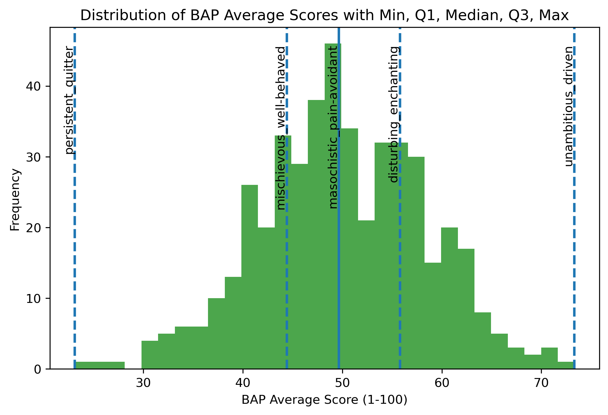
For “unambitious_driven,” the average ratings are skewed toward driven, suggesting that characters are generally perceived as driven rather than unambitious. In contrast, “persistent_quitter” shows ratings concentrated closer to persistent, indicating that characters are more often characterized as persistent than as quitters. Together, these patterns suggest that in movie character development, traits such as being driven and persistent are more commonly emphasized or recognized by viewers than their opposing traits.
Plotted a histogram of the standard deviations within each BAP column.
Image(filename = "visualizations/bap_std_histogram.png")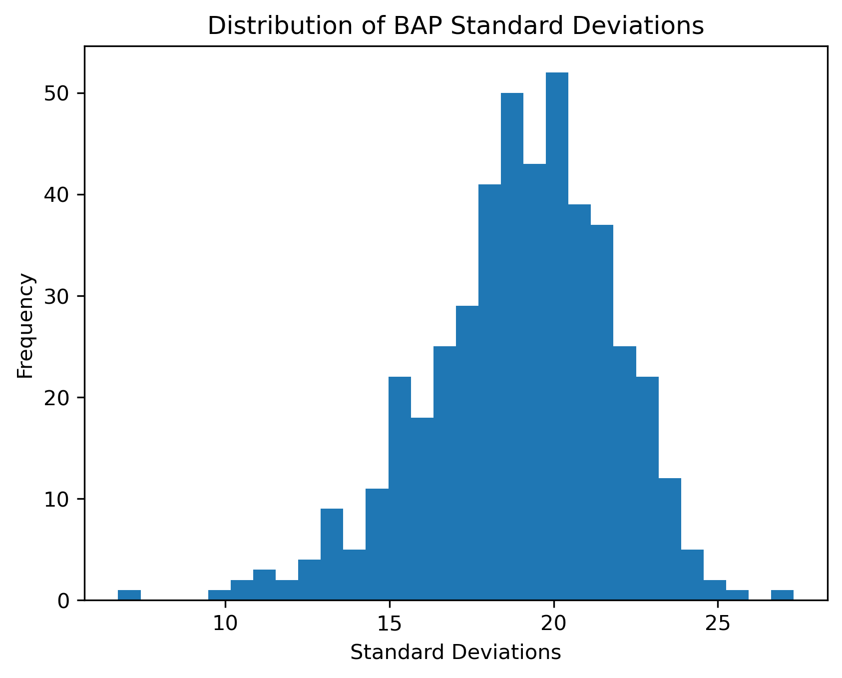
The BAP ratings seem to vary from their means as much as approximately 28 scores to about 6. While on average they seem to vary close to about 20 scores. BAPs like “right-brained left-brained” or “Coke Pepsi” might not be very hard to discern characters that are on the polar opposites since they aren’t very intuitive as to what a more right-brained person looks like or a more “Coke” person is. On the other hand, for BAPs like “masculine feminine” or “parental childlike”, it is clearer and more intuitive to understand what more female than male means or what being more of a main character than side character looks like.
Plotted a correlation matrix between the BAP columns for a better understanding of the data before PCA.
Image(filename = "visualizations/default_correlation_map.png")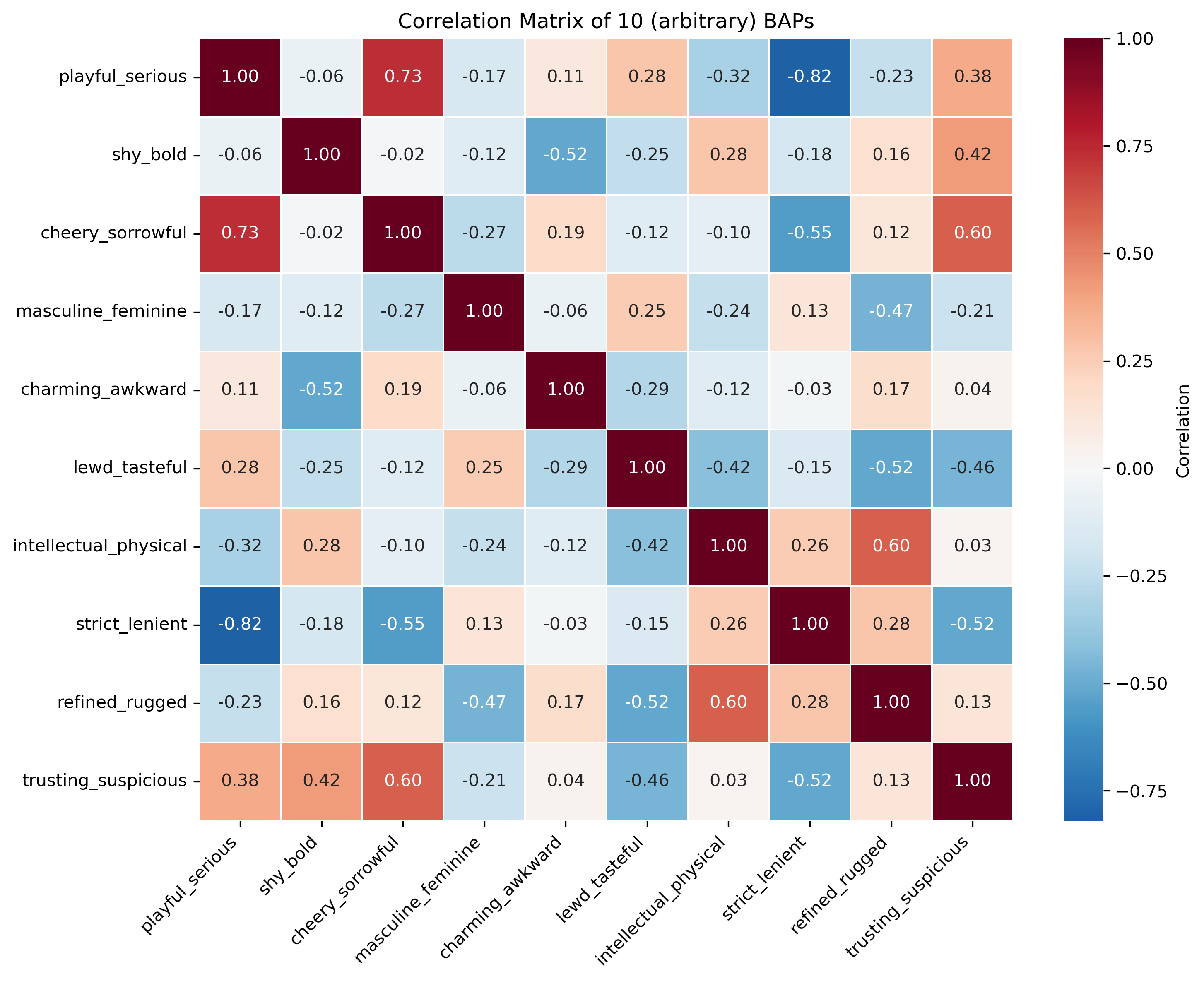
In the correlation matrix, there are some variables that are very strongly correlated like “playful_serious” and “strict_lenient” are strongly negatively correlated assuming they have a linear relationship. This makes sense because people who are more playful are likely also lenient while those who are serious are strict. There are also a lot of close to uncorrelated variables like “trusting_suspicious” and “intellectual_physical” where they don’t seem to be related in a certain way.
Average rankings distribution for the top 10 sources or media sources with the most number of characters.
Image(filename = "visualizations/average_rankings_for_top10_sources.png")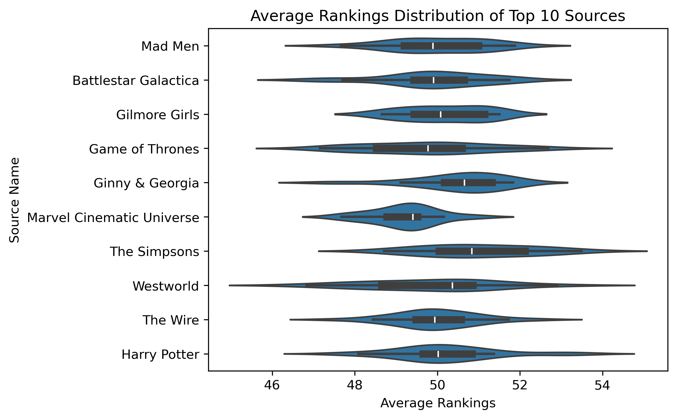
While the average rankings roughly center around 50, characters in the Marvel Cinematic Universe have, on average, slightly lower ratings than average, while Westworld characters have higher ratings than the average.
Finding Associations
From the exploratory data analysis, we found fun associations that fans would likely find amusing or obvious. But there are also associations that may suggest deeper cultural norms about how certain categories of people are depicted in fiction. In this section, we look at four dimensions that speak to important demographic categories: straight_queer, young_old, masculine_feminine, and rich_poor. It is important to note that, by categorizing characters based on respondents’ ratings on these dimensions, we are assessing how perceptions of these categories are related to perceptions of other dimensions.
Image(filename = "visualizations/selected_dim_correlation_map.png")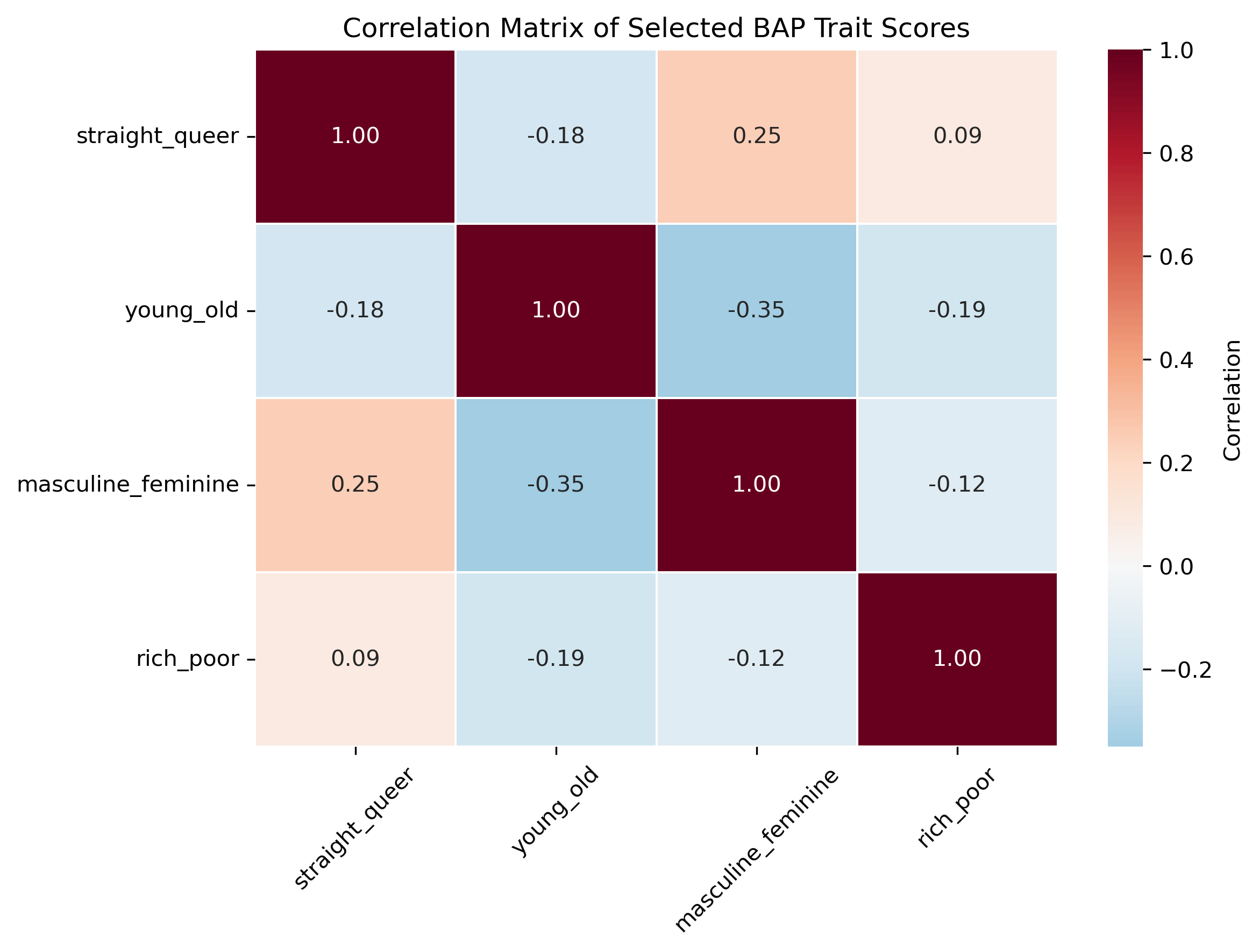
We see that the features are not very strongly (pairwise) correlated with each other. This is good as we do not need to reduce dimensionality.
While these dimensions are not strongly (pairwise) correlated with each other, they may be correlated with other dimensions in the data set. To start, we can standardize the data and create a 500x500 correlation matrix. While this would be a mess to visualize, we can select our target dimensions and see if if they are highly correlated with any other dimensions.
target_corr_df = pd.read_csv("data/target_correlations.csv")
target_corr_dfBy social sciences standards, there are some strong correlations here. For example, straight_queer is inversely correlated with androgynous_gendered, which suggests that the more queer a character is, the more likely their depiction is androgynous. However, these correlations are not controlling for the influence of other dimensions. We can instead calculate the partial correlations, which show us correlations between dimensions while controlling for other dimensions.
target_pcorrs_df = pd.read_csv("data/target_partial_corr.csv")
target_pcorrs_dfThese coefficients are far less suggestive of strong relationships. However, given how many redundant dimensions we have in the data, this might simply be an issue of too much noise and too unsophisticated of a method. We can revist these questions after doing some dimension reduction in the next section.
Identifying Archetypes
In the Vermont Computational Story Lab’s analysis of the same dataset, they used “dimension reduction” to identify 6 key dimensions in the data that create 12 archetypes. However, because the replication code has not been made available, it is unclear what techniques they used to reduce the dimensionality of the data. In this section, we employ a mixture of principal component analysis (PCA), Gaussian mixture model (GMM), and hierarchical agglomerative clustering (HAC) to propose some potential archetypes.
PCA
For PCA, it is important to scale variable values because we are comparing Euclidean distances. Technically, all of our variables should already be on the same scale, but this will become more important when we get to the self-organizing map, so we will scale them here for consistency.
We will assess how many components we should have. The first technique plotted below is adapted from this tutorial. The author recommends that the number of components chosen should account for 95% of the variance.
Image(filename = "visualizations/cumulative_variance_PCA.png")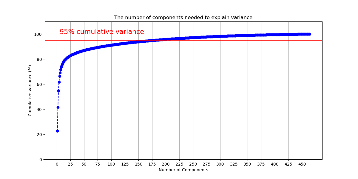
The figure shows that we will need 177 components to capture 95% of the variance. 177 components does not reduce the dimensionality of the data very much. Thus, we flipped the figure to see how much variance is captured by each component. Given our previous results, we will limit this to the first 50 components to make the data more legible.
Image(filename = "visualizations/scree_plot_PCA.png")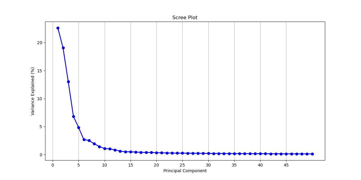
Another common dimension reduction strategy is to only select components from before the curve begins to flatten out, which would be 5 components. At 5 components, 66.4% of the variance is captured.
To see which of the 500 dimensions contribute the most to each of the components, we can access the component loadings. Loadings tell us both the magnitude and direction of a given dimension, which, together indicate how the dimension contributes to the presence of a given component: A (relatively) larger, positive loading suggests that that dimension contributes more to the presence of that component. We retrieve the top 10 loadings from the first 15 components. We swap their values (e.g., 0.091049) for the dimension’s name (e.g., rude_respectful). Then, we add the loading’s sign (positive or negative) to the name.
pca_loadings_10 = pd.read_csv("data/pca_comp_loadings.csv")
pca_loadings_10To interpret this we can look at PC1’s top 2 loadings come from the dimensions +rude_respectful and -angelic_demonic. This tells us that both dimensions contribute to the presence of PC1 but that they inversely relate. This means someone who scores highly on respectful would be expected to score lower on demonic. When interpreting the dimensions, remember that the right-hand side corresponds to the higher scores, and the left-hand side corresponds to the lower scores. Interpreting the loadings, the first five components seem to get at the following dichotomies:
“good” vs “bad”
“serious” vs “silly”
“bland” vs “cool”
“refined” vs “rough”
“smart” vs “strong”
There are some components which speak to the questions posed in finding associations. PC4 contains rich_poor, as well as other dimensions indicating wealth. The component would seem to suggest that the rich are depicted as more “manicured”, “preppy”, and “lavish” as opposed to “scruffy”, “punk-rock”, and “frugal”. Past the first five components, the groupings of terms become harder to interpret and their explanatory power diminishes, but we see young_old make an appearance in PC7. Here “old” is aligned with “repulsive”, “comedic”, and “happy.” PC10 brings together masculine_feminine and straight_queer, with queerness and feminity aligned. They are also aligned with “cat-person”, “androgynous”, “asexual”, “side-character”, and, oddly enough, “German.”
Clustering: Gaussian Mixture Models
While PCA reduces dimensions, it does not cluster our data. However, we can use PCA to cluster the data with reduced noise from excess dimensions. One way of clustering our data is through a Gaussian Mixture Model. This model is ideal for its probabilistic nature: It would allow us to have “soft” clusters, with some characters occupying the boundaries between multiple archetypes. To quickly test this model out, we can input the 177 components of our PCA which explain 95% of the variance and cluster our characters into one of two groups. We can plot each character on a scatterplot with the first two principle components as the axes.
Image(filename = "visualizations/GMM_2_components.png")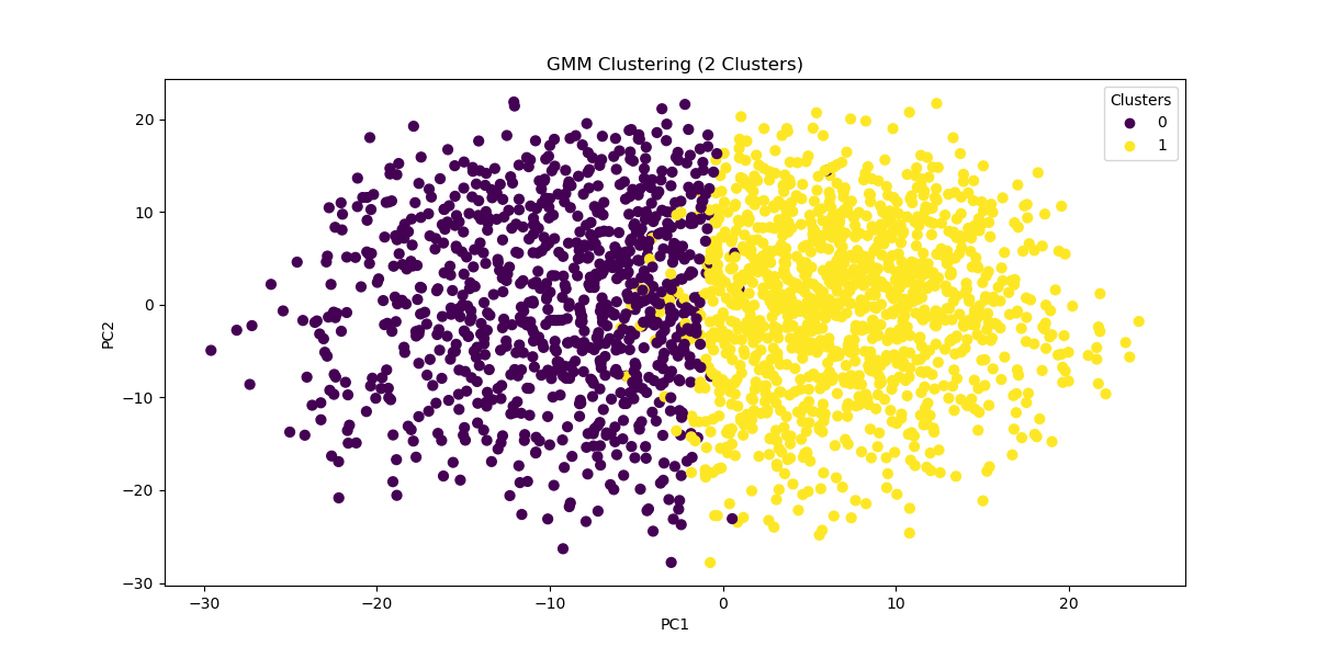
The clusters separate fairly well. Now let’s take a look at what characters fall into each group. This might help us assess the viability of this method. We can assign cluster labels to the characters and input each character’s score on the 177 components. We chose characters from the Batman Universe for this analysis.
char_gmm2 = pd.read_csv("data/char_gmm2.csv")
char_gmm2Looks like all the good guys (assigned 1) and all the bad guys (assigned 0) are clustered together except Bruce Wayne. To try and interpret this division, we can take the mean of every PCA component for each of the clusters and then reverse the dimensionality reduction. We reinstantiate our PCA with only the first 177 components to do this. Next, we go through each cluster and retrieve the original dimensions with the highest absolute average. We still care about the direction of the sign though, so we print the mean value alongside the dimension name. It turns out that the two clusters are just the opposite of one another: Cluster 0 is defined by being more rude while Cluster 1 is more respectful.
Cluster 0:
rude_respectful -0.90848501438952
wholesome_salacious 0.9102933704149965
poisonous_nurturing -0.9118241177741682
naughty_nice -0.9135515721810906
angelic_demonic 0.9268963015825046
Cluster 1:
rude_respectful 0.6677719310792272
wholesome_salacious -0.6691011433128735
poisonous_nurturing 0.6702263023455916
naughty_nice 0.6714960487331381
angelic_demonic -0.6813049455018976
Now let’s do the same analysis but with more initial clusters:
Image(filename = "visualizations/GMM_6_components.png")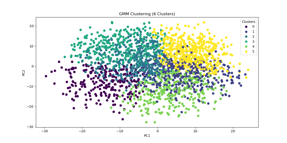
With 6 clusters we find these cluster labels and interpretations:
char_gmm6 = pd.read_csv("data/char_gmm6.csv")
char_gmm6Cluster 2:
maverick_conformist -0.9778032087470556
spicy_mild -0.9970935439066825
wild_tame -0.9998038258299139
obedient_rebellious 1.0265447574944488
tattle-tale_fuck-the-police 1.0449993578169918
Cluster 3:
open-minded_close-minded 1.3675472277193188
democratic_authoritarian 1.3748352164453137
protagonist_antagonist 1.3889034862462442
cruel_kind -1.4111948253980606
soulless_soulful -1.4644891912684297
Cluster 5:
ludicrous_sensible 1.02199526147885
stable_unstable -1.0272058392071326
factual_exaggerating -1.0313798432912424
deranged_reasonable 1.0352385760146183
juvenile_mature 1.0615990016387764
With three times as many clusters, Bruce Wayne’s allies all remain in the same group (one now defined by being stable, sensible, factual, reasonable, and mature). Meanwhile, Harvey Dents splits off, and The Joker and Bruce Wayne stay together. This suggests that, perhaps, a better technique for clustering the data would be hierarchical.
Hierarchical Clustering
While hierarchical clustering will employ different methods for differentiating clusters and thus, is unlikely to replicate the clusters found through GMM, this is actually the reason for attempting to cluster the data with it: Perhaps what we need is a hierarchical approach to show how certain categories break down. We will start by plotting a dendrogram to give us a sense of the shape of the data.
Image(filename = "visualizations/HCA_complete_dendrogram.png")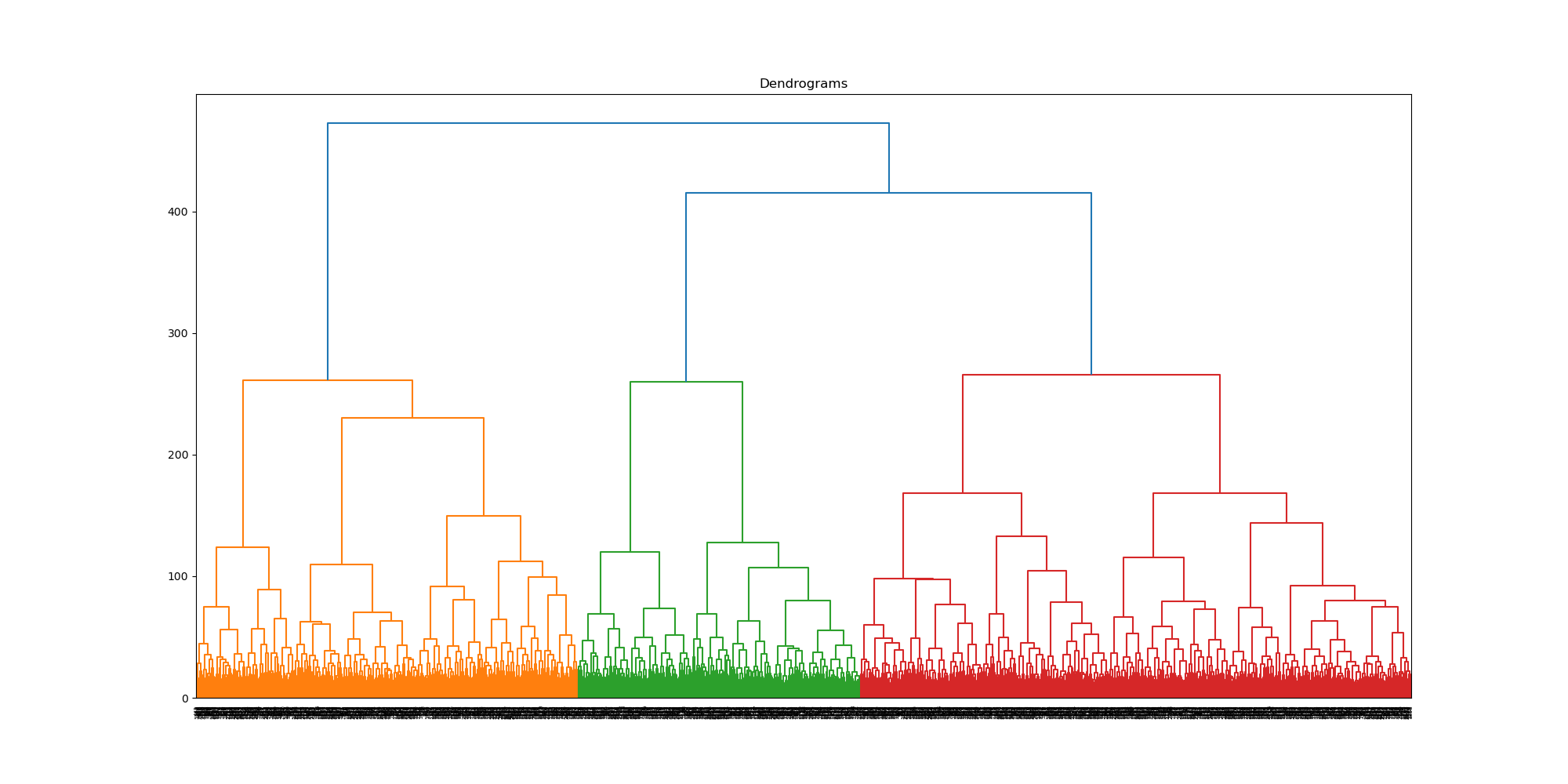
As we did with GMM we will divide the data into two clusters, but this time using agglomerative clustering. We are still using the 177 components identified earlier. We can compare the cluster labels to GMM assigned to each character.
gmm_vs_hier = pd.read_csv("data/gmm_vs_hier.csv")
gmm_vs_hierSeems like The Joker is all alone in his own cluster. To see what differentiates these two groups, we can create a new dataframe with the clusters as columns and the original dimensions as rows—just like we did with our PCA. Repurposing that code, we can figure out which dimensions differentiate the clusters based on their average scores.
hier_cluster_dim = pd.read_csv("data/hier_cluster_dim.csv")
hier_cluster_dimThe highest scoring dimensions are the difference between order and chaos, scandalous and proper, and caution and impulse. The Joker certainly seems to make sense on the side of chaos.
Now we can enter into the hierarchy again, this time once 7 groups have been created, and run the same analysis.
gmm_vs_hier7 = pd.read_csv("data/gmm_vs_hier7.csv")
gmm_vs_hier7hier_cluster_dim7 = pd.read_csv("data/hier_cluster_dim7.csv")
hier_cluster_dim7The Joker stays on his lonesome, but his new cluster is defined by “adventurous”, “rebellious”, and “fuck the police”—so it seems like an appropriate place for him. Meanwhile, the agents of order have been split into two camps: butler Alfred Pennyworth and district attorney / love interest Rachel Dawes are “warm”, “angelic”, and “nurturing”, while vigilante Bruce Wayne, lawyer-turned-killer Harvey Dent, and police commissioner James Gordon are all “rational”, “no nonsense”, and “mature.”
For a final attempt at interpreting the data, we can label each “leaf” of the tree with the most prominent dimension and cut the tree off to visualize the hierarchy. The code is minorly adapted from stack overflow.
Image(filename = "visualizations/HCA_2cluster_dendrogram.png")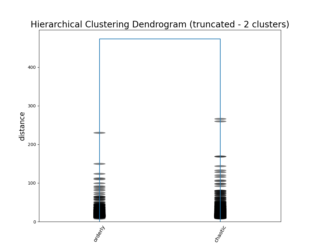
Image(filename = "visualizations/HCA_7cluster_dendrogram.png")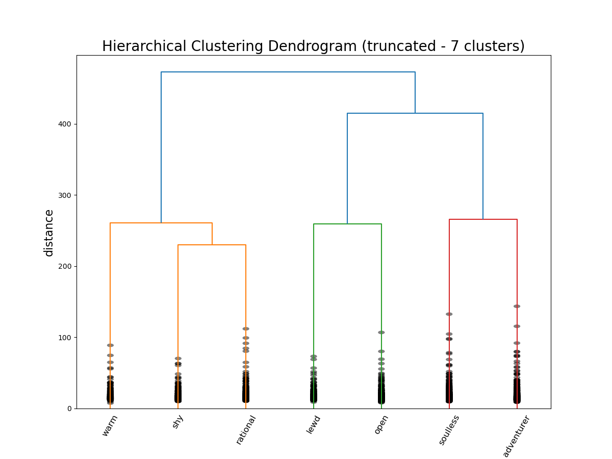
We certaintly did not produce the same archetypes as the Vermont Computational Story Lab (CSL). Their 6 major dimensions are roughly approximated by our 5 components derived via PCA, but they were not exact. These axes seemed more true to what we might consider “archetypes”: PC5, for example, described tropes of characters defined by their brains or their brawn, which corresponds to CSL’s “brute vs geek” dimension. When it came to GMM, the major distinctions didn’t capture the heros vs the villains, but seemed to capture a general personality difference. The more psychological aspects of the character archetypes became clear with the hierarchical clustering. This makes sense given the fact that Open Psychometrics relies on personality-based metrics—it’s even in the name.
With some interpretive leverage, we could identity the major differentiation between characters as whether or not they are agents of order or chaos—an important distinction in how characters move plots along. On the side of order, there are characters defined by their warmth and kindness, their shyness and meekness, or their wise rationality. On the side of chaos, there are characters defined by their perversion, their gregariousness and charm, their cruelty and villainy, and their wild rebelliousness.
Conclusion
From exploratory data analysis, most characters were rated near the middle on many traits. This means that no single personality trait usually defined a character on its own. However, some traits such as being driven, persistent, and serious appeared more frequently across characters, suggesting that fiction often emphasizes active and motivated personalities.
When looking at the demographic traits “queer_straight”, “young_old”, “masculine_feminine”, and “rich_poor”, not much insights came from their pairwise correlations, but rather from patterns revealed through PCA analysis. This method showed that the characters are mainly portrayed using multitude of traits rather than isolated characteristics. Characters rated wealthier tended to be more polished, refined, and extravagant, while poorer characters were associated with being rougher or more practical. Older characters tended to be associated with traits like repulsive, comedic, and happy. Lastly, queerness and femininity were tied together and aligned with traits such as androgynous, asexual, side-character, and cat-person.
Among the methods used to identify archetypes, hierarchical clustering produced the most interpretable results. While PCA helped reveal underlying dimensions and GMM identified broad personality splits, hierarchical clustering most clearly distinguished characters based on psychological and moral roles. In particular, it highlighted a divide between characters associated with order and those associated with chaos. This structure aligns closely with common storytelling archetypes, suggesting that hierarchical clustering was effective in uncovering fictional character groupings.
Author Contributions
Peter Forberg:
I downloaded the data, created additional data files based on the codebook, and generated an outline for our project. I setup the structure of the analysis notebooks. For 1-intro_exploration.ipynb, I created a cleaned dataframe and provided some initial exploration. For 2-finding_associations.ipynb, I added additional analyses using correlation matrices (specifically to identify top correlations and then introduce dimension control). For 3-identify_archetypes.ipynb, I tested multiple clustering and dimension reduction techniques (including some abandoned factor analysis and self-organizing maps). I wrote/adapted the code for PCA, GMM, and HAC. I contributed to the environment.yml and the README.md.
Neha Suresh:
I worked primarily on the 1-intro_exploration.ipynb notebook, where I used the cleaned data from Peter to create EDA charts and explore correlations. I continued exploring correlations in 2-finding-associations.ipynb to generate a correlation map for the selected BAP features. I also modularized some of the EDA code into functions to make it easier for my team to reuse and extend. Additionally, I saved all visualizations in the visualizations folder and the processed data in the data folder for easy access and reusability across notebooks. Finally, I updated the environment.yml file based on the imports I used and tested the environment to ensure all notebooks I worked on run smoothly.
Harish Raghunath: I worked on designing separating the function definitions through separate files and packages, as well as making the Makefile and researching the license to use for our group. For the functions, I took the modularized functions Neha and Peter designed in the notebooks and made an installable package called “finaltools” which contains the tests and functions with relevant docstrings for the python file and each function. Furthermore, I designed the tests which verify the functionality of the functions defined, and read through the LICENSE guide to choose the right license for the project.
Sofia Lendahl:
I worked on consolidating all the analysis notebooks into the main.ipynb notebook. I organized this notebook into a research paper format, saved key dataframes from the analysis notebook into the data folder, displayed key figures from the visualizations folder, summarized key findings, and cleaned up the verbiage. I also created a binder link and attached the badge to the README.md, created the MyST site and deployed to GitHub Pages, added the .gitignore, and rendered all of the analysis notebooks and main notebook each as a separate PDF file using MyST and stored them in the pdf_builds folder.
- Dodds, P. S. (2025). Archetypometrics dataset. Zenodo. 10.5281/ZENODO.16953724
- Ramasubramanian, S., Riewestahl, E., & Ramirez, A. (2023). Race and Ethnic Stereotypes in the Media. In Oxford Research Encyclopedia of Communication. Oxford University Press. 10.1093/acrefore/9780190228613.013.1262
- Rodriguez, J. A. (2019). Lesbian, Gay, Bisexual, Transgender, and Queer Media: Key Narratives, Future Directions. Sociology Compass, 13(4), e12675. 10.1111/soc4.12675
- Mendes, K., & Carter, C. (2008). Feminist and Gender Media Studies: A Critical Overview. Sociology Compass, 2(6), 1701–1718. 10.1111/j.1751-9020.2008.00158.x
- Johfre, S. (2020). What Age Is in a Name? Sociological Science, 7, 367–390. 10.15195/v7.a15
- Kozlowski, A. C., Taddy, M., & Evans, J. A. (2019). The Geometry of Culture: Analyzing the Meanings of Class through Word Embeddings. American Sociological Review, 84(5), 905–949. 10.1177/0003122419877135