Part 2: Simple Text Processing - Tokenization, Lemmatization, Word Frequency, Vectorization (20 pts)
Part 2: Simple Text Processing - Tokenization, Lemmatization, Word Frequency, Vectorization (20 pts)
Now we will start working on simple text processing using the SpaCy package and the same dataset as Part 1. The package should already be included in the environment.yml. However, we will also need to download en_core_web_sm, an English language text processing model. To do this, while having your sotu environment activated, run the following:
python -m spacy download en_core_web_smNow, you should be good to go!
Some important definitions:
Token: a single word or piece of a word
Lemma: the core component of a word, e.g., “complete” is the lemma for “completed” and “completely”
Stop Word: a common word that does not add semantic value, such as “a”, “and”, “the”, etc.
Vectorization: representing a document as a vector where each index in the vector corresponds to a token or word and each entry is the count.
In this section, we will explore the most common tokens and lemmas throughout different slices of the speech data. We will also develop vectorization representations of the speeches.
The core steps are:
Process speeches using the SpaCy nlp module
Analyze Tokens vs Lemmas:
Create a list of all tokens across all speeches that are not stop words, punctuation, or spaces.
Create a second list of the lemmas for these same tokens.
Display the top 25 for each of these and compare.
Analyze common word distributions over different years:
Create a function that takes the dataset and a year as an input and outputs the top n lemmas for that year’s speeches
Compare the top 10 words for 2023 versus 2019
Document Vectorization:
Train a Term Frequency-Inverse Document Frequency (TF-IDF) vectorization model using your processed dataset and scikit learn
Output the feature vectors
Helpful Resources:
Step 1: Process speeches using the SpaCy nlp module
import spacy
spacy.cli.download("en_core_web_sm")
# importing all of the necessary packages
import pandas as pd
import matplotlib.pyplot as plt
import seaborn as sns
import spacy
import mpld3
from tqdm import tqdm
from collections import Counter
from sklearn.decomposition import PCA
from matplotlib.colors import LogNorm
nlp = spacy.load("en_core_web_sm")# make a path for the outputs
from pathlib import Path
OUTPUT_DIR = Path("outputs")
OUTPUT_DIR.mkdir(exist_ok=True)# load the data
sou = pd.read_csv("data/SOTU.csv")
sou_21cen = sou[sou["Year"] >= 2000].reset_index(drop=True)
sou_21cenStep 2: Analyze Tokens vs Lemmas
processed_speech = []

for text in tqdm(sou_21cen["Text"], desc="Processing"):
    doc = nlp(text)
    processed_speech.append(doc)
Processing: 100%|██████████| 25/25 [00:24<00:00, 1.01it/s]
# displaying the top tokens
tokens = []

for doc in processed_speech:
    for token in doc:
        if not token.is_stop and not token.is_punct and not token.is_space:
            tokens.append(token.text.lower())

token_counts = Counter(tokens)
top_tokens = token_counts.most_common(25)
top_tokens
[('america', 816),
('people', 637),
('american', 582),
('new', 530),
('years', 439),
('americans', 437),
('world', 425),
('year', 406),
('country', 369),
('jobs', 348),
('tonight', 344),
('work', 324),
('know', 323),
('let', 320),
('congress', 317),
('nation', 311),
('time', 301),
('help', 282),
('need', 266),
('tax', 255),
('president', 247),
('economy', 243),
('like', 241),
('right', 240),
('want', 237)]# displaying the top lemmas
lemmas = []
for doc in processed_speech:
for token in doc:
if not token.is_stop and not token.is_punct and not token.is_space:
lemmas.append(token.lemma_.lower())
lemma_counts = Counter(lemmas)
top_lemmas = lemma_counts.most_common(25)
top_lemmas[('year', 845),
('america', 816),
('people', 639),
('american', 587),
('work', 557),
('new', 532),
('job', 486),
('country', 435),
('americans', 432),
('world', 426),
('know', 395),
('nation', 388),
('help', 378),
('need', 353),
('time', 351),
('tonight', 344),
('child', 332),
('let', 326),
('congress', 317),
('come', 301),
('family', 296),
('good', 294),
('right', 282),
('million', 274),
('want', 264)]# comparison between the top tokens and top lemmas
tokens_w, tokens_c = zip(*top_tokens)
lemmas_w, lemmas_c = zip(*top_lemmas)
compare_df = pd.DataFrame({
"Token": tokens_w,
"Token Count": tokens_c,
"Lemma": lemmas_w,
"Lemma Count": lemmas_c
})
compare_dfIn the token list, words like “year” and “years” appear separately, so their counts are split across two entries (439 for years and 406 for year). After lemmatization, these are merged into the single lemma “year”, which now shows a higher combined count of 845, giving a clearer picture of how often this concept appears. A similar pattern shows up for “job/jobs”. In the token table, jobs appears with a count of 348, but once we normalize to the lemma “job”, the total frequency rises to 486. These examples illustrates how lemmas group different grammatical forms together, revealing the underlying themes more clearly than raw tokens.
Step 3: Analyze common word distributions over different years:
# making a function to find the top lemmas by year
def top_lemmas_by_year(df, year, n=10):
    docs = nlp.pipe(df[df["Year"] == year]["Text"])
    lemmas = [
        token.lemma_.lower()
        for doc in docs
        for token in doc
        if not token.is_stop and not token.is_punct and not token.is_space
    ]
    return Counter(lemmas).most_common(n)
# top 10 lemmas for 2024
top_2024 = top_lemmas_by_year(sou_21cen, 2024, 10)
top_2024[('president', 58),
('year', 45),
('america', 44),
('american', 34),
('people', 33),
('$', 33),
('member', 32),
('want', 29),
('audience', 29),
('know', 29)]# top 20 lemmas for 2023 and 2017
top_2023 = top_lemmas_by_year(sou_21cen, 2023, 20)
top_2017 = top_lemmas_by_year(sou_21cen, 2017, 20)top_2023[('year', 58),
('go', 56),
('let', 45),
('know', 40),
('people', 39),
('job', 38),
('america', 36),
('come', 33),
('law', 33),
('pay', 33),
('american', 31),
('$', 31),
('president', 30),
('look', 27),
('world', 25),
('folk', 24),
('nation', 24),
('audience', 23),
('work', 23),
('right', 23)]top_2017[('american', 34),
('america', 29),
('country', 26),
('nation', 21),
('great', 20),
('new', 19),
('year', 19),
('world', 18),
('job', 15),
('people', 15),
('americans', 14),
('united', 13),
('tonight', 13),
('states', 12),
('work', 12),
('child', 12),
('want', 12),
('time', 12),
('citizen', 11),
('right', 11)]# comparing the top lemmas and their counts for 2017 and 2023
lem23, cnt23 = zip(*top_2023)
lem17, cnt17 = zip(*top_2017)
compare_2017_2023_df = pd.DataFrame({
"2023 Lemma": lem23,
"2023 Count": cnt23,
"2017 Lemma": lem17,
"2017 Count": cnt17
})
compare_2017_2023_dfWe see 2023 uses more economy-focused language (e.g., job, pay), whereas 2017 emphasizes national identity (american, america, country).
# making bar graphs for the top lemmas in 2017 and 2023
sns.set_theme(style="dark")
compare_fig, axes = plt.subplots(2, 1, figsize=(10, 8))

sns.barplot(
    ax=axes[0],
    x="2017 Lemma",
    y="2017 Count",
    data=compare_2017_2023_df,
)
axes[0].set_title("2017 State of the Union Most Frequent Words")
axes[0].set_xlabel("Word")
axes[0].set_ylabel("Count")
axes[0].tick_params(axis='x', rotation=45)

sns.barplot(
    ax=axes[1],
    x="2023 Lemma",
    y="2023 Count",
    data=compare_2017_2023_df,
)
axes[1].set_title("2023 State of the Union Most Frequent Words")
axes[1].set_xlabel("Word")
axes[1].set_ylabel("Count")
axes[1].tick_params(axis='x', rotation=45)

plt.tight_layout()
plt.show()

mpld3.save_html(compare_fig, str(OUTPUT_DIR / "compare_2017_2023_bars.html"))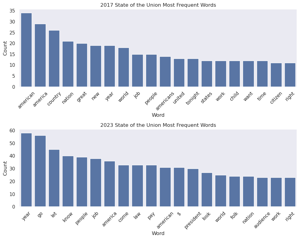
Step 4: Document Vectorization
from sklearn.feature_extraction.text import TfidfVectorizer
# Convert speech text column into a list of documents
raw_docs = sou["Text"].to_list()
# Create and fit the TF-IDF vectorizer on the speeches
tfidf_model = TfidfVectorizer()
tfidf_vectors = tfidf_model.fit_transform(raw_documents=raw_docs)
# Get the list of vocabulary words learned by TF-IDF
feature_names = tfidf_model.get_feature_names_out()
tfidf_dense = tfidf_vectors.toarray()
# Turn the TF-IDF results into a DataFrame
tfidf_df = pd.DataFrame(
    tfidf_dense,
    columns=feature_names,
    index=sou["Year"]
)
tfidf_df
pca = PCA(n_components=2)
pca_result = pca.fit_transform(tfidf_df)
pca_df = pd.DataFrame(
    pca_result,
    columns=["PC1", "PC2"],
    index=tfidf_df.index
)
pca_df# making a scatterplot of the vectorized speeches principal components
pca_scatter_fig, pca_scatter_ax = plt.subplots(figsize=(10, 6))
pca_scatter_ax.scatter(pca_df["PC1"], pca_df["PC2"], alpha=0.8)
pca_scatter_ax.set_title("Plot of Vectorized Speeches Principal Components", fontsize=14)
pca_scatter_ax.set_xlabel("Principal Component 1")
pca_scatter_ax.set_ylabel("Principal Component 2")
plt.show()
mpld3.save_html(pca_scatter_fig, str(OUTPUT_DIR / "vectorized_speeches_pca_scatter.html"))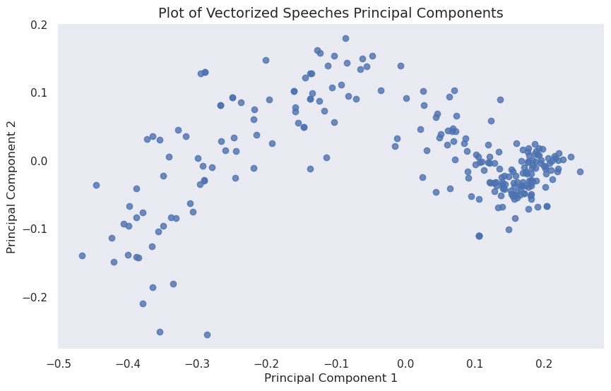
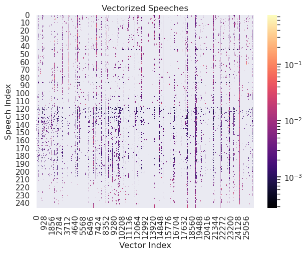
# making a heatmap of the vectorized speeches
tfidf_dense = tfidf_vectors.toarray()
vectorized_heatmap_fig, vectorized_heatmap_ax = plt.subplots(figsize=(7, 5))

sns.heatmap(
    tfidf_dense,
    cmap="magma",
    norm=LogNorm(),
    ax=vectorized_heatmap_ax
)

vectorized_heatmap_ax.set_title("Vectorized Speeches")
vectorized_heatmap_ax.set_xlabel("Vector Index")
vectorized_heatmap_ax.set_ylabel("Speech Index")

plt.show()

vectorized_heatmap_fig.savefig(
    OUTPUT_DIR / "vectorized_speeches_heatmap.png",
    dpi=300,
    bbox_inches="tight"
)
word_list = ['year',
 'america',
 'people',
 'american',
 'work',
 'new',
 'job',
 'country',
 'americans',
 'world'] # top ten most common words through whole corpus
# get each word's index number using the .vocabular_ attributed of vectorizer
word_nums = [tfidf_model.vocabulary_[w] for w in word_list]# get their IDF score by using .idf_ at the indices from the previous step
idf_score = [tfidf_model.idf_[i] for i in word_nums]# get the tf_idf score for the first speech
tf_idf = [tfidf_vectors[0, i] for i in word_nums]pd.DataFrame({
"Word": word_list,
"IDF Score": idf_score,
"TF-IDF Score": tf_idf
})
Overall, the top words seem to be strongly centered around national identity and employment. Out of the top ten words, the word with the highest IDF score is “job.” The word “america” has the highest TF-IDF score.