RQ1: Which socioeconomic and geographic factors most strongly predict food affordability in California? - Final Project: Food Affordability in California

Approach¶

To identify which socioeconomic and geographic factors most strongly predict food affordability in California, we focus on a small set of interpretable predictors:

Socioeconomic: median_income
Geographic: region_name
Demographic: race_eth_name

Why filter to geotype == "PL"? We restrict the analysis to place-level observations to keep the unit of analysis consistent (cities/towns/CDPs) and avoid mixing geographic levels that may have different variance structures.

Modeling choice: We compare a baseline (mean-only) model to Ridge regression models using 1-, 2-, and 3-feature subsets. Ridge is a linear model that remains interpretable while stabilizing estimates when one-hot encoding categorical predictors.

Important note on leakage / interpretability: We intentionally did not usecost_yr as a predictor here because affordability_ratio is conceptually tied to cost and income. Including variables that directly define the outcome can inflate predictive performance without answering “which contextual factors matter most.”

import numpy as np
import pandas as pd
from pathlib import Path
import matplotlib.pyplot as plt

from sklearn.model_selection import train_test_split
from sklearn.dummy import DummyRegressor
from sklearn.metrics import mean_absolute_error, r2_score
from utils.model_utils import rmse, make_ridge_model, eval_model_rq1

RANDOM_STATE = 159
np.random.seed(RANDOM_STATE)

DATA_PATH = Path("./data/food_affordability.csv")
OUT_DIR = Path("./outputs"); OUT_DIR.mkdir(exist_ok=True)
FIG_DIR = Path("./figures"); FIG_DIR.mkdir(exist_ok=True)

df = pd.read_csv(DATA_PATH)

drop_cols = [
    "version", "ind_definition", "ind_id", "reportyear",
    "LL95_affordability_ratio", "UL95_affordability_ratio",
    "se_food_afford", "rse_food_afford",
    "county_name", "county_fips", "region_code",
    "ave_fam_size"
]
df = df.drop(columns=drop_cols, errors="ignore")

df.shape

(14365, 11)

TARGET = "affordability_ratio"
FULL_FEATURES = ["region_name", "race_eth_name", "median_income"]

# Filter to Place-level only
df_pl = df[df["geotype"] == "PL"].copy()

# Keep only rows where target and all full features exist
df_pl = df_pl.dropna(subset=[TARGET] + FULL_FEATURES).copy()

print("Rows after PL filter + dropna:", df_pl.shape[0])
df_pl[FULL_FEATURES + [TARGET]].head()

Rows after PL filter + dropna: 3003

# one consistent split for fair comparison across models
X = df_pl[FULL_FEATURES].copy()
y = df_pl[TARGET].copy()

X_train, X_test, y_train, y_test = train_test_split(
    X, y, test_size=0.2, random_state=RANDOM_STATE
)

X_train.shape, X_test.shape

((2402, 3), (601, 3))

import itertools

features = FULL_FEATURES  # ["region_name", "race_eth_name", "median_income"]
results = []

# Baseline model
dummy = DummyRegressor(strategy="mean")
dummy.fit(X_train, y_train)
pred_dummy = dummy.predict(X_test)
results.append({
    "model": "Dummy(mean)",
    "features": "",
    "RMSE": rmse(y_test, pred_dummy),
    "MAE": mean_absolute_error(y_test, pred_dummy),
    "R2": r2_score(y_test, pred_dummy),
})

# Models using 1 feature, 2 features, and all 3 features
for k in [1, 2, 3]:
    for subset in itertools.combinations(features, k):
        subset = list(subset)
        name = f"Ridge(log1p y) | {', '.join(subset)}"
        model = make_ridge_model(subset, X_train)

        out = eval_model_rq1(
            name,
            model,
            X_train[subset], X_test[subset],
            y_train, y_test
        )
        out["features"] = ", ".join(subset)
        results.append(out)

metrics_rq1 = pd.DataFrame(results).sort_values("RMSE")
metrics_rq1

metrics_rq1.to_csv(OUT_DIR / "rq1_pl_subset_models_metrics.csv", index=False)

plt.figure(figsize=(10, 4))
plt.barh(metrics_rq1["model"][::-1], metrics_rq1["RMSE"][::-1])
plt.xlabel("RMSE (test)")
plt.title("Model comparison across feature subsets")
plt.savefig(FIG_DIR / "rq1_pl_subset_models_rmse.png", dpi=150, bbox_inches="tight")
plt.show()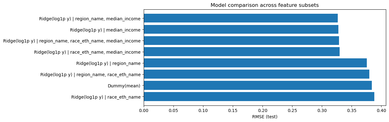

Across the tested feature subsets, models that include median income perform best. The top-performing specification uses region_name + median_income, achieving RMSE ≈ 0.3267 and R² ≈ 0.2705 on the test set. Using median_income alone is nearly as good (RMSE ≈ 0.3276, R² ≈ 0.2664), suggesting that income is the dominant predictor in this setup.

Adding race_eth_name does not improve performance here (the 3-feature model has slightly worse RMSE/R² than the best 2-feature model). Meanwhile, region_name alone performs much worse (R² near 0.03), indicating that regional labels by themselves explain little unless income is included.

Overall, these results indicate that median income is the strongest predictor of food affordability, with region contributing a small additional gain beyond income in this place-level sample.